My journey of pursuing Deeplearning.ai Course @Coursera - Course 1, Week 2

 

Course 1:  Neural Networks and Deep Learning

Week 2: Neural Networks Basics

About : Learn to set up a machine learning problem with a neural network mindset. Learn to use vectorization to speed up your models.

Key Concepts

• Build a logistic regression model, structured as a shallow neural network
• Implement the main steps of an ML algorithm, including making predictions, derivative computation, and gradient descent.
• Implement computationally efficient, highly vectorized, versions of models.
• Understand how to compute derivatives for logistic regression, using a backpropagation mindset.
• Become familiar with Python and Numpy
• Work with iPython Notebooks
• Be able to implement vectorization across multiple training examples

Lec 1 : Binary Classification

Logistic regression : Type of Binary Classification Problem

y ---> Output Label

Unroll all the Pixels to a Long Vector

If img is 64*64 pixels --> The tot dim of the vector will be 64*64*3 = 12288

nx = 12288

n = Denotes Dimension of this feature vector

(x,y) --> trg eg

m = trg eg

We will stack X in columns and Y also in Columns.

Useful convention...  Take data associated with diff trg eg and stack in different columns

Part 2 : Logistic Regression

if X is a pic what is the probability it is a cat pic?

- w is  a nx dim vector

One thing we could try, that does not work is to take Output = w^T x + b ... (Linear Regression)

But we need values between 0 and 1, hence it will not work!

So we will take sigmoid of the output

We take z to denote (w^T x + b)

- b is a real number

When z is large, Sigmoid of z becomes = 1

When z is large -ve number, Sigmoid of z becomes = 0

When we program, we will keep the parameter w and b separate, where B corresponds to an inner-spectrum. We will not use any of the convention written in red. 

Part 3 : Logistic Regression Cost Function

Loss error(function) --> 1/2 of Squared error

But the optimisation problem shall become non convex, So we end up with optimization problem with multiple local optima. So gradient descent might not get the global optimum. 

So we don't do this in Logistic Regression.

So we use this in Logistic regression: 

Loss Function :-

---------------------

L(y_hat,y) = - (ylog (y_hat) + (1-y) log (1 - (y_hat)))

-------------------------------------

Some intuition regarding this,

If we are using squared error we would want the squared error to be as min as possible, and with the Logistic Regression Loss function we want the same, to be as small as possible.

 

So the loss function, Defines how well we are doing in one single dataset, while 

Cost Function : Defines how well we are doing in the entire training eg.

                        J(w,b) = 1/m (Sum(Loss Function)) , i.e.

J(w,b)=m1​∑i=1m​L(yhat(i),y(i))=−m1​∑i=1m​(y(i)logyhat(i)+(1−y(i))log(1−yhat(i)))

The cost function is the avg of the loss functions of the entire training set, its the cost of our parameters.... We need to minimize this Cost Function

    

Part 4: Gradient Descent

The cost function is :

J(w,b)=m1​∑i=1m​L(yhat(i),y(i))=−m1​∑i=1m​(y(i)logyhat(i)+(1−y(i))log(1−yhat(i)))

So J(w,b) is a convex function.

We initialize J(w,b) as a dot, and for logistic regression almost any initialization method works.

So Gradient Descent starts at the initial point and then takes a step in the steepest downhill direction.

And after two iterations of gradient descent you might step there, 

three iterations and so on. 

I guess this is now hidden by the back of the plot until eventually, hopefully you 

converge to this global optimum or get to something close to the global optimum. 

So this picture illustrates the gradient descent algorithm. 

Were going to take the value of w and update it, going to use colon equals to represent updating w. So set w to w minus alpha, times, and this is a derivative dJ(w)/dw. 

We will repeatedly do that until the algorithm converges. 

So couple of points in the notation, alpha here, is the learning rate, and controls how big a step we take on each iteration or gradient descent. 

The derivative  is basically the update or the change you want to make to the parameters w. When we start to write code to implement gradient descent, we're going to use the convention that the variable name in our code

dw will be used to represent this derivative term. So when you write code you write something like w colon equals w minus alpha times dw. And so we use dw to be the variable name to represent this derivative term.

In logistic regression, your cost function is a function of both w and b. So in that case, the inner loop of gradient descent, that is this thing here, this thing you have to repeat becomes as follows. You end up updating w as w minus the learning rate times the derivative of J(w,b) respect to w. And you update b as b minus the learning rate times the derivative of the cost function in respect to b. So these two equations at the bottom are the actual update you implement. 

Part 5 and 6: Derivatives and Examples

The slope of this function is equal to three, meaning that whatever is the value of a, if you increase it by 0.001, the value of f of a goes up by three times as much. So, this function has a safe slope everywhere. One way to see that is that, wherever you draw this little triangle. The height, divided by the width, always has a ratio of three to one. So,  this gives us a sense of what the slope or the derivative of a function means for a straight line, where in this example the slope of the function was three everywhere. 

But if f(a) = a^2, the slope is different t different points.

So the tips from the videos are:-

• The derivative of the function just means the slope of a function and the slope of a function can be different at different points on the function. In our first example where f(a) = 3a those a straight line. The derivative was the same everywhere, it was three everywhere. For other functions like f(a) = a² or f(a) = log(a), the slope of the line varies. So, the slope or the derivative can be different at different points on the curve. So that's a first take away. Derivative just means slope of a line.
• Second takeaway is that if you want to look up the derivative of a function, you can flip open your calculus textbook or look up Wikipedia and often get a formula for the slope of these functions at different points. 

Part 7: Computation graph

So, the computation graph comes in handy when there is some distinguished or some special output variable, such as J in this case, that you want to optimize. And in the case of a logistic regression, J is of course the cost function that we're trying to minimize. 

One step of backward propagation on a computation graph yields derivative of final output variable.

Part 8 : Derivatives with a Computation Graph

So the key takeaway from this video, from this example, is that when computing derivatives and computing all of these derivatives, the most efficient way to do so is through a right to left computation following the direction of the red arrows. And in particular, we'll first compute the derivative with respect to v. And then that becomes useful for computing the derivative with respect to a and the derivative with respect to u. And then the derivative with respect to u, for example, this term over here and this term over here. Those in turn become useful for computing the derivative with respect to b and the derivative with respect to c. 

Here, the coding convention dvar represents the derivative of a final output variable with respect to various intermediate quantities.

Part 9: Logistic Regression Gradient Descent

Recapping LR,

Now for the backward propagation,

Because what we want to do is compute derivatives with respect to this loss, the first thing we want to do when going backwards is to compute the derivative of this loss with respect to, the script over there, with respect to this variable A. So, in the code, you just use DA to denote this variable. 

Here's the Derivative of the Sigmoid function:

https://towardsdatascience.com/derivative-of-the-sigmoid-function-536880cf918e

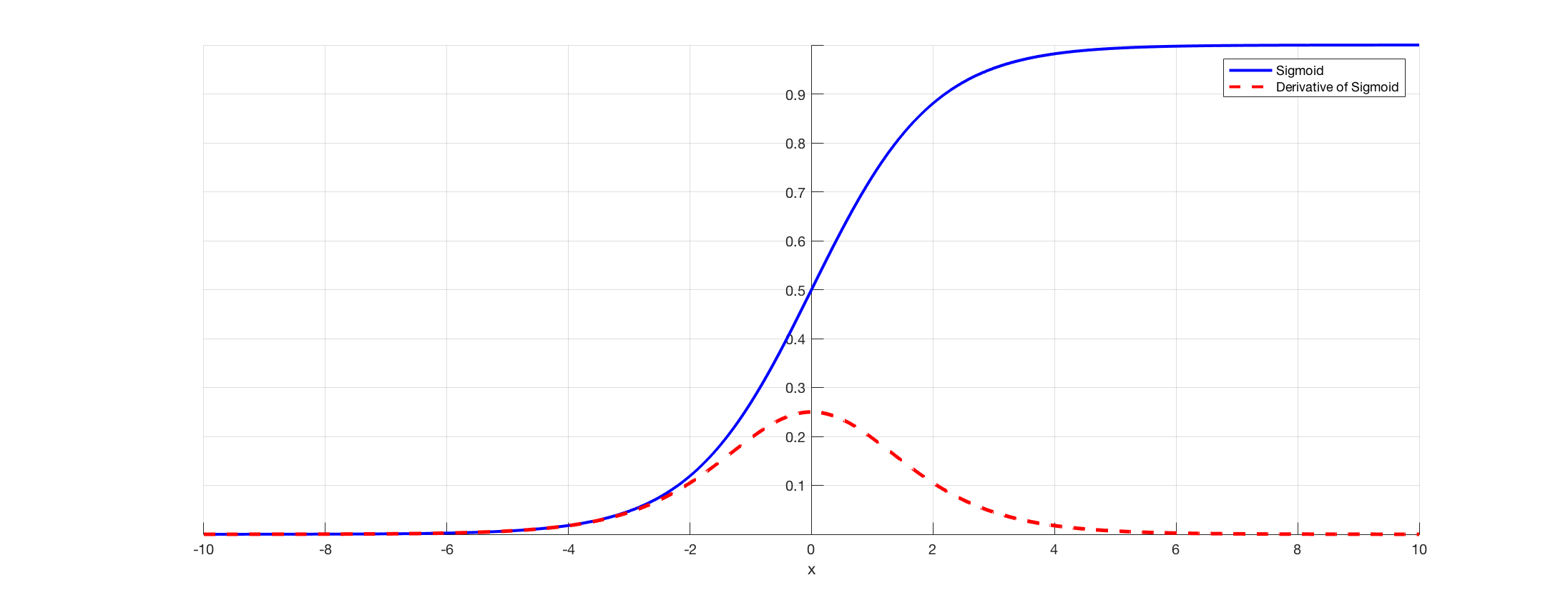
                                                Graph of Sigmoid and the derivative of the Sigmoid function

Derivation of DL/dz  : 

https://www.coursera.org/learn/neural-networks-deep-learning/discussions/weeks/2/threads/ysF-gYfISSGBfoGHyLkhYg

$dz=a-y$

Part 10: Gradient Descent on m Examples

We, notice that dw_1 and dw_2 do not have a superscript i, because we're using them in this code as accumulators to sum over the entire training set. 

Whereas in contrast, dz_i here, this was dz with respect to just one single training example. So, that's why that had a superscript i to refer to the one training example, i that is computerised. So, having finished all these calculations, to implement one step of gradient descent, you will implement w_1, gets updated as w_1 minus the learning rate times dw_1, w_2, ends up this as w_2 minus learning rate times dw_2, and b gets updated as b minus the learning rate times db, where dw_1, dw_2 and db were as computed. 

Finally, J here will also be a correct value for your cost function. So, everything on the slide implements just one single step of gradient descent, and so you have to repeat everything on this slide multiple times in order to take multiple steps of gradient descent.

But it turns out there are two weaknesses with the calculation as we've implemented it here, which is that, 

to implement logistic regression this way, you need to write two for loops. The first for loop is this for loop over the m training examples, and the second for loop is a for loop over all the features over here. So, in this example, we just had two features; so, n is equal to two and x equals two, but maybe we have more features, you end up writing here dw_1 dw_2, and you similar computations for dw_t, and so on delta dw_n. So, it seems like you need to have a for loop over the features, over n features. When you're implementing deep learning algorithms, you find that having explicit for loops in your code makes your algorithm run less efficiency. We will use VECTORIZATION to reduce for loops usage :)

Part 11 &12 : Vectorization and Examples

 Vectorization is basically the art of getting rid of explicit folders in your code

Non-Vectorized vs Vectorized version:-

In vectorized version, we use 

np.dot(w,x) + b instead of running a loop

Tip: Avoid using for loops

                        Non-Vectorised                                                            Vectorised

Part 13: Vectorizing Logistic Regression

X is a n_x by m matrix.

Make a 1 by m matrix [ z1,z2,....z_m] ---> w^t X + [b1,b2.....bm]   (make it Z)

So this W transpose will be a row vector like that. And so this first term will evaluate to W transpose X1, W transpose X2 and so on, dot, dot, dot, W transpose XM, 

Python implementation: - 

Z = np.dot(w.T , X) + b                      { Python automatically converts the real no. b to a 1 by m row vector  } ;)   --> This feature is called Broadcasting in Python

Part 14: Vectorizing Logistic Regression's Gradient Output

 what we did was we computed dz1 for the first example, which could be a1 minus y1 and then dz2 equals a2 minus y2 and so on. And so on for all M training examples. So, what we're going to do is define a new variable, dZ is going to be dz1, dz2, dzm. Again, all the D lowercase z variables stacked horizontally. So, this would be 1 by m matrix or alternatively a m dimensional row vector. 

So with one line of code, we are able to do everything. :) 

i.e, db = 1/m * np.sum(dz)

      dw = 1/m * X * dz

So, we've just done forward propagation and back propagation, really computing the predictions and computing the derivatives on all M training examples without using a for loop. And so the gradient descent update then would be you know W gets updated as w minus the learning rate times dw which was just computed above and B is update as B minus the learning rate times db. Sometimes is putting colons to that to denote that as is an assignment. And with this, we have just implemented a single iteration of gradient descent for logistic regression.

 

But if we want to implement multiple iterations as a gradient descent then you still need a full loop over the number of iterations. So, if you want to have a thousand iterations of gradient descent, you might still need a full loop over the iteration number. 

Part 15: Broadcasting in Python

To add a bit of detail this parameter, (axis = 0), means that you want Python to sum vertically. So if this is axis 0 this means to sum vertically, where as the horizontal axis is axis 1. So be able to write axis 1 or sum horizontally instead of sum vertically. 

We might not even use .reshape() command. And technically, after this first line of codes cal, the variable cal, is already a one by four matrix. So technically you don't need to call reshape here again, so that's actually a little bit redundant.

IMP NOTE : 

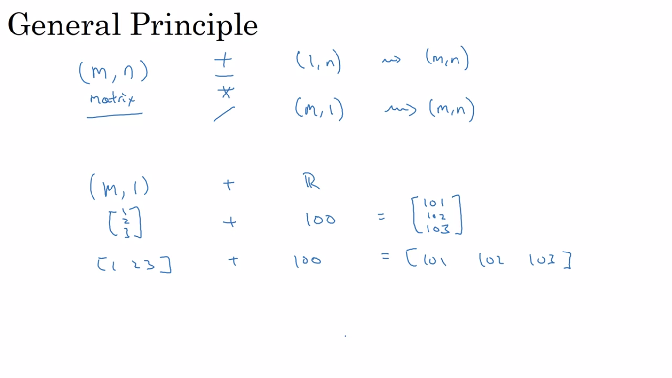
Here's the more general principle of broadcasting in Python. If you have an (m,n) matrix and you add or subtract or multiply or divide with a (1,n) matrix, then this will copy it n times into an (m,n) matrix. And then apply the addition, subtraction, and multiplication of division element wise.

If conversely, you were to take the (m,n) matrix and add, subtract, multiply, divide by an (m,1) matrix, then also this would copy it now n times. And turn that into an (m,n) matrix and then apply the operation element wise. Just one of the broadcasting, which is if you have an (m,1) matrix, so that's really a column vector like [1,2,3], and you add, subtract, multiply or divide by a row number. So maybe a (1,1) matrix. So such as that plus 100, then you end up copying this real number n times until you'll also get another (n,1) matrix. And then you perform the operation such as addition on this example element-wise. And something similar also works for row vectors.

Part 16: A note on python/numpy vectors

We should always use either ...

a = np.random.randn(5,1)

or 

a = np.random.randn(1,5)

But, not the rank 1 code, i.e a = np.random.randn(5)

We can also use the assert(a.shape == (5,1)) or the reshape func, as 

they take O(1) time and are very cheap.

Part 17 : Explanation of logistic regression cost function

We said that we want to interpret y hat as the p( y = 1 | x). So we want our algorithm to output y hat as the chance that y = 1 for a given set of input features x. So another way to say this is that if y is equal to 1 then the chance of y given x is equal to y hat. And conversely if y is equal to 0 then

the chance that y was 0 was 1- y hat, right? So if y hat was a chance, that y = 1, then 1- y hat is the chance that y = 0. 

 And there's a negative sign there because usually if you're training a learning algorithm, you want to make probabilities large whereas in logistic regression we're expressing this. We want to minimize the loss function. So minimizing the loss corresponds to maximizing the log of the probability. So this is what the loss function on a single example looks like.

And so in statistics, there's a principle called the principle of maximum likelihood estimation, which just means to choose the parameters that maximizes this thing. Or in other words, that maximizes this thing. Negative sum from i = 1 through m L(y hat ,y) and just move the negative sign outside the summation. So this justifies the cost we had for logistic regression which is J(w,b) of this. And because we now want to minimize the cost instead of maximizing likelihood, we've got to rid of the minus sign. And then finally for convenience, to make sure that our quantities are better scale, we just add a 1 over m extra scaling factor there. But so to summarize, by minimizing this cost function J(w,b) we're really carrying out maximum likelihood estimation with the logistic regression model. Under the assumption that our training examples were IID, or identically independently distributed.

                                                            :) Completing Week 2 :)